GeoJSON: Import and Styling with VTS-Browser-JS
This tutorial provides a step by step guide how to import and visualize sample GeoJSON data with VTS-Browser-JS.
In detail we’ll take a look how to display the VTS browser on a webpage. Next we’ll load some GeoJSON data and display them. And finally we’ll take a sneak peek into the possibilities of visual style customization.
You can find the code and a live demo of this tutorial on JSFiddle.
GeoJSON
GeoJSON is an open standard format designed for representing simple geographical features, along with their non-spatial attributes, based on JavaScript Object Notation. You can view the specs here.
Displaying the browser
To display the VTS Browser, add the necessary CSS and
JavaScript resources and create a div with an id like map-div.
<!DOCTYPE html>
<html lang="en">
  <head>
      <link rel="stylesheet" href="https://cdn.melown.com/libs/vtsjs/browser/v2/vts-browser.min.css"/>
      <script src="https://cdn.melown.com/libs/vtsjs/browser/v2/vts-browser.min.js"></script>
  </head>
  <body>
     <div id="map-div" style="width:100%; height:100%;"></div>
     <script>
         <!-- add your js code here -->
     </script>
  </body>
</html>
Now that we’ve prepared our HTML structure we can add some JavaScript code to make the browser run.
var browser = null;
var renderer = null;
var map = null;
var geodata = null;

function startDemo() {
    browser = vts.browser('map-div', {
        map: 'https://cdn.melown.com/mario/store/melown2015/map-config/melown/VTS-Tutorial-map/mapConfig.json',
        position : [ 'obj', -122.48443455025, 37.83071587047, 'float', 0.00, 19.04, -49.56, 0.00, 1946.45, 55.00 ]
    });

    //check whether browser is supported
    if (!browser) {
        console.log('Your web browser does not support WebGL');
        return;
    }

    //callback once is map config loaded
    browser.on('map-loaded', onMapLoaded);
}

function onMapLoaded() {
  // geojson loading here
}

startDemo();
We created a map in place of the map-div and set the map parameter
to point to a map configuration we prepared in Melown Cloud for this purpose.
You can create your own map in Melown Cloud. We set the
position
to San Francisco Golden Gate Bridge. You can discover more about
browser configuration parameters in
documentation.
Once the map loads we can start with
importing a GeoJSON. We achieve this by using the callback function
onMapLoaded and registering it to listen for the map-loaded event.
You should now see the following:
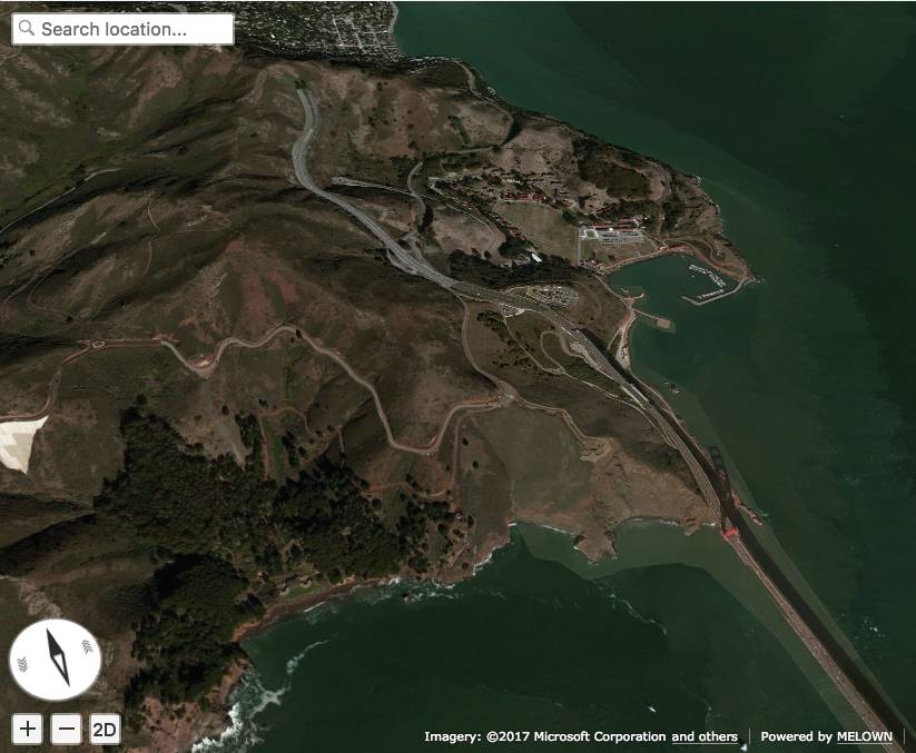
Initial image
Adding GeoJSON data
Let’s assume we have the following GeoJSON data containing a sample trek trough Golden Gate Bridge Vista Point.
var json = {
    "type": "FeatureCollection",
    "features": [
        {
            "type": "Feature",
            "geometry": {
                "type": "Point",
                "coordinates": [-122.48347, 37.82955],
            },
            "properties": {
                "title": "Golden Gate Bridge Vista Point",
            }
        },
        {
            "type": "Feature",
            "properties": {},
            "geometry": {
                "type": "LineString",
                "coordinates": [
                    [-122.48369693756, 37.83381888486],
                    [-122.48344236083, 37.83317489144],
                    [-122.48335253015, 37.83270036637],
                    [-122.48361819152, 37.83205636317],
                    [-122.48404026031, 37.83114119107],
                    [-122.48404026031, 37.83049717427],
                    [-122.48348236083, 37.82992094395],
                    [-122.48356819152, 37.82954808664],
                    [-122.48507022857, 37.82944639795],
                    [-122.48610019683, 37.82880236636],
                    [-122.48695850372, 37.82931081282],
                    [-122.48700141906, 37.83080223556],
                    [-122.48751640319, 37.83168351665],
                    [-122.48803138732, 37.83215804826],
                    [-122.48888969421, 37.83297152392],
                    [-122.48987674713, 37.83263257682],
                    [-122.49043464660, 37.83293762928],
                    [-122.49125003814, 37.83242920781],
                    [-122.49163627624, 37.83256478721],
                    [-122.49223709106, 37.83337825839],
                    [-122.49378204345, 37.83368330777]
                ]
            }
        }
    ]
}
The data contains two features. One point and one line represented by a list of coordinates. In addition to geometry data every feature can have custom properties such as a title, as in the current example. We’ll take advantage of this later in the tutorial.
To load the data into the browser we need to implement the onMapLoaded()
function mentioned earlier:
function onMapLoaded() {
    map = browser.map;

    // create geodata object
    geodata = map.createGeodata();

    // import GeoJSON data
    geodata.importGeoJson(json);

    geodata.processHeights('node-by-precision', 62, onHeightsProcessed);
}
We create a geodata object with map.createGeodata() that we can
use to import a GeoJSON with geodata.importGeoJson(json, <mode = float>). During the
import, the height of features is interpreted either as above the terrain
(float mode, default) or above ellipsoid (fix mode).
If heights are missing, 0 is assumed and therefore float should be used.
geodata.processHeights(...) must be called for every float data to
display them correctly.
At the moment VTS Browser does not support importing polygons as a feature type.
function onHeightsProcessed() {

    var style = {
        // add your style here
    };

    // make free layer
    var freeLayer = geodata.makeFreeLayer(style);

    // add free layer to the map
    map.addFreeLayer('geodatatest', freeLayer);

    // add free layer to the list of free layers
    // which will be rendered on the map
    let view = map.getView();
    view.freeLayers.geodatatest = {};
    map.setView(view);
}
The function onHeightsProcessed() creates a free layer out of the GeoJSON
data and adds our custom style to it. Now you have all the data rendered,
but it’s still invisible because we need to first add some styles to
the newly created layers.
Basic styling
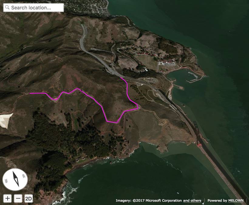
Let’s start with a really basic one. We’ll omit point data for now and just display a magenta line. To do so, let’s change the style object to the following:
var style = {
    layers: {
        "track-line" : {
            "filter" : ["==", "#type", "line"],
            "line": true,
            "line-width" : 4,
            "line-color": [255,0,255,255]
        }
    }
};

Basic styling
style now contains the property layers which works as a container
component for all style layers we want to use. Direct children of
layers can have arbitrary names. In the example above we’ve added
one style layer and named it track-line. A style layer can have
multiple properties that you can find
here.
The most important one is filter.
Filter is used to select features from the GeoJSON to which we want to apply
a set of display rules described in the current style layer. In our example we
are applying display rules to all lines. This filter selects everything
from features where type equals line. The "line":true means
we want to display the current feature as a line. line-width specifies
line width. And finally we set line color to magenta with line-color,
which accepts RGBA values as an array.
You can find a comprehensive documentation for styles here.
Advanced styling
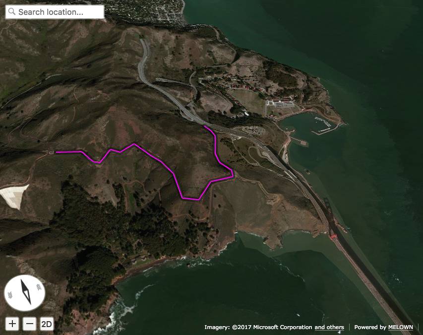
You may have noticed that the line dives under the surface. This happens due
to interpolation of line height between points. We can fix this by adding
zbuffer-offset to the track-line layer. Try to add
"zbuffer-offset": [-0.5, 0, 0] and see the difference.
Displayed track with zbuffer-offset
Now we’ll add a shadow to the line’s visual style.
var style = {
    layers: {
        "track-line" : {
            "filter" : ["==", "#type", "line"],
            "line": true,
            "line-width" : 4,
            "line-color": [255,0,255,255],
            "zbuffer-offset" : [-0.5,0,0],
            "z-index" : -1
        },
        "track-shadow" : {
            "filter" : ["==", "#type", "line"],
            "line": true,
            "line-width" : 20,
            "line-color": [0,0,0,120],
            "zbuffer-offset" : [-0.5,0,0],
        }
    }
};
Added track shadow
Okay, so far we have managed to visualize a line feature. But if we go back to our sample GeoJSON data we notice that it contains a feature of type point as well. We’ll focus on visualizing that one now.
We’ll make the point appear as a green circle with it’s title displayed above it.
var style = {
    "constants": {
        "@icon-marker": ['icons', 6, 8, 18, 18]
    },
    "bitmaps": {
        "icons": 'http://maps.google.com/mapfiles/kml/shapes/placemark_circle.png'
    },
    "layers": {
         "track-line" : {
            "filter" : ["==", "#type", "line"],
            "line": true,
            "line-width" : 4,
            "line-color": [255,0,255,255],
            "zbuffer-offset" : [-0.5,0,0],
            "z-index" : -1
        },
        "track-shadow" : {
            "filter" : ["==", "#type", "line"],
            "line": true,
            "line-width" : 20,
            "line-color": [0,0,0,120],
            "zbuffer-offset" : [-0.5,0,0],
        },

        // added new style for point
        "place" : {
                "filter":["==", "#type", "point"],

                "icon": true,
                "icon-source": '@icon-marker',
                "icon-color": [0,255,0,255],
                "icon-scale": 2,
                "icon-origin": 'center-center',

                "label": true,
                "label-size": 19,
                "label-source": "$title",
                "label-offset": [0,-20],
                "zbuffer-offset" : [-1,0,0]
        }
    }
};
We’ve added two new properties to style. The bitmap.icons defines
a URL with overlay icon resource. In constants we define
variables that can be reused troughout the style object. Here we define
the constant @icon-marker and select a rectangle out of icons PNG.
The first two numbers in the array define the top left corner and the last two numbers
the bottom right corner in image coordinates.
We’ve also added a new layer group place to layers. Notice that
now we have used a different filter to select all points instead. For
icon-source we have used the defined constant. Notice that for
label-source we used $title. This means that the contents of the point’s
title property should be used as a label. The rest of the style
properties are self-explanatory.
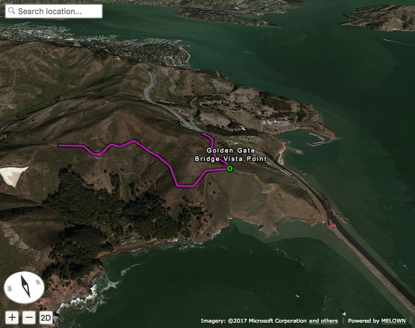
Track with point
That’s it for now, you’ve made it to the end :)
In the next tutorial we’ll take a look at loading extra data from the URL and extending the track.